Implementing SKALA-1.1 in vibe-qc: from a neural functional to molecular and periodic SCF

How an AI-assisted implementation turned Microsoft’s nonlocal neural exchange-correlation model into an experimental, reproducible provider for molecular and periodic density-functional theory, and where the validation boundary still lies.

Late one evening last week, I asked Codex to implement Microsoft’s SKALA exchange-correlation functional in vibe-qc. By the next morning, the first implementation was done. Over the following days we concentrated on the work that makes an implementation usable: reading the source paper, defining a general interface, adding periodic density projection, checking checkpoint provenance, writing tests, documenting the restrictions, and preparing examples that fail closed when a requested method is not yet scientifically supported.

The result is now part of vibe-qc as an experimental functional. The first molecular adapter shipped in v0.15.158; v0.15.160 expanded the experimental periodic infrastructure, including GPW, GAPW, and AICCM/four-centre entrances. Follow-up hardening on main tightens the high-level four-centre option forwarding and ECP guards for the next release.

This article is not an accuracy announcement for solids. It is an implementation report: what SKALA is, why it required a different XC interface, which molecular and periodic routes are present, what has been tested, and what has deliberately not yet been claimed.

What is different about SKALA?

Most exchange-correlation functionals used in electronic-structure programs have a local interface. At each quadrature point they consume a density and perhaps its gradient, Laplacian, or kinetic-energy density. A library such as libxc can evaluate those points in batches because the result at one point does not depend explicitly on all the others.

SKALA-1.1, introduced by Luise and co-workers at Microsoft Research, is different. It is a learned, nonlocal functional. In the authors’ notation its energy has the form

E_xc^θ[ρ] = −(3/4)(6/π)^1/3 ∫ [ρ_α^4/3 + ρ_β^4/3] f_θ(x[ρ]; r) dr.

The model starts from seven semilocal channels: the two spin densities, the squared gradient magnitude of each spin density, the kinetic-energy density of each spin channel, and the squared gradient magnitude of the total density. Those features are log-transformed and passed through a local branch in both spin orderings, with the results averaged to enforce spin-order invariance.

Nonlocality enters through a hierarchy of atom-centred coarse points. The architecture uses 16 radial functions and spherical harmonics through ℓ = 3, mixes equivariant coarse features, applies symmetric contractions for higher-body correlations, and repeats a downsample/process/upsample sequence three times. A scaled sigmoid constrains the enhancement factor to the interval stated by the authors. The complete checkpoint has 385,217 parameters, 331,265 of them in the local branch: compact by current machine-learning standards, but qualitatively different from a pointwise functional.

The original paper reports, under its own reference geometries and protocols, a GMTKN55 WTMAD-2 of 2.80 kcal mol⁻¹, an S22 mean absolute error of 0.14 kcal mol⁻¹, and W4-17 mean absolute errors of 0.92 kcal mol⁻¹ for the 183 single-reference cases and 1.23 kcal mol⁻¹ over all 200 cases. These are the authors’ benchmark results, not results produced by vibe-qc.

The important engineering consequence is simple: one grid point is no longer a sufficient unit of evaluation.

A full-grid XC provider

The most reusable part of this work is not a special if functional == "skala" branch. It is a versioned full-grid provider contract.

The host code assembles the complete atom-major quadrature grid and sends the provider the coordinates, final and atomic weights, atom ownership, molecular or periodic metadata, and the fields ρ_σ, ∇ρ_σ, and τ_σ. The provider returns one integrated exchange-correlation energy together with adjoints with respect to every input feature.

Those adjoints are then projected into the AO matrix:

V_μν,σ^xc = ∂E_xc/∂P_μν,σ.

Expanded by the chain rule, this contains contributions through the density, density gradient, and kinetic-energy density. One easily missed detail is that the returned adjoints already contain the quadrature weights. Multiplying by the weights again in the AO projection would give a smooth-looking but wrong potential.

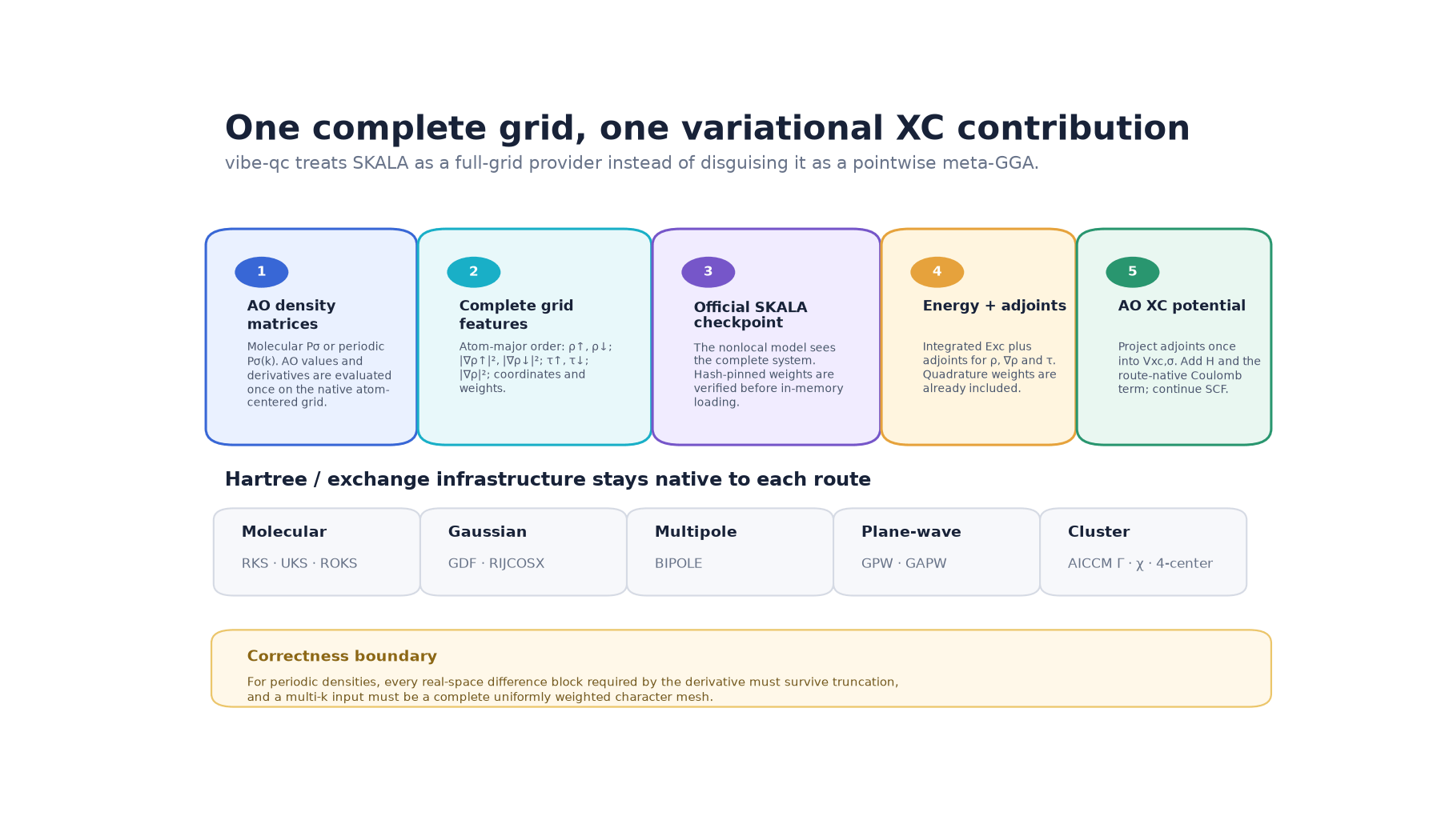
For a fixed geometry, the molecular path is consequently a two-pass operation:

1. Build every required feature over the complete grid.
2. Evaluate SKALA once and retain its integrated energy and adjoints.
3. Project those adjoints into the RKS, UKS, or ROKS AO potential and continue the SCF cycle.

The separation is useful beyond SKALA. Any future nonlocal model that can provide an integrated energy and consistent feature derivatives can use the same host boundary without becoming entangled with the molecular or periodic Coulomb backend.

Reproducibility starts before the first matrix multiplication

vibe-qc does not bundle Microsoft’s checkpoint or import another quantum-chemistry program at runtime. The optional skala extra provides the independent adapter and the compatible PyTorch runtime. The official CPU checkpoint is fetched on demand from its immutable upstream revision.

The contract records the expected byte size, SHA-256 digest, source revision, feature order, grid profile, protocol version, and D3 metadata. The bytes are verified immediately before TorchScript deserialization and are loaded from memory, avoiding a check-then-load race. Calculation manifests retain the checkpoint, execution, grid, data-type, and chunking provenance.

The current execution envelope is deliberately narrow: Linux CPU, Python 3.11 through 3.13, and PyTorch 2.12 or 2.13. A missing or mismatched checkpoint is an error, not an invitation to continue with a nearby file.

This also defines the redistribution boundary. vibe-qc ships its MPL-2.0 adapter and a hash-pinned on-demand fetch mechanism; it does not ship the model weights or Microsoft’s runtime. Our repository audit found no copyright or training-data-license blocker to that adapter/fetch design. It did not clear redistribution of the checkpoint itself, and it is not a patent freedom-to-operate opinion or an indication of Microsoft endorsement.

Periodic DFT is not molecular DFT with a unit cell label

For a periodic calculation, the spin density is assembled from lattice-resolved AO blocks. Schematically,

ρ_σ(r) = Σ_g Σ_μν P_μν^σ(g) χ_μ(r) χ_ν(r − g),

with analogous expressions for the density gradient and kinetic-energy density. After the model is evaluated, its adjoints must be differentiated back into the same real-space lattice blocks and then Bloch-summed into V_xc(k).

The central correctness condition is difference closure. If the active AO cells contain translations a and s, then the XC domain must retain every difference g = s − a required by the derivative. Truncating that difference set can yield an apparently converged energy paired with a nonvariational Fock matrix.

Multi-k support introduces another constraint. The transformation between k-space density matrices and real-space lattice blocks is a discrete Fourier transform. A complete, uniformly weighted Monkhorst-Pack character mesh has that structure; an arbitrary weighted list of k-points does not. vibe-qc therefore rejects meshes that cannot be expanded into the required complete set instead of silently treating them as equivalent.

The same separation of responsibilities is important for plane-wave-assisted methods. In GPW and GAPW, the native FFT or augmented Hartree builder remains active, while SKALA sees one complete AO density. GAPW deliberately does not evaluate the neural functional independently on smooth, hard, and soft components and then add those numbers: nonlocality makes that decomposition unjustified.

Current route map

The figure below summarizes the implementation state on current main. Every periodic row remains experimental and currently assumes zero-temperature occupations. “Integrated” means that the provider path exists and has contract-level tests; it does not mean that materials-level accuracy has been established.

In prose, the current scope is:

• molecular RKS, UKS, and ROKS fixed-geometry single-point SCF;
• GDF RKS/UKS at Γ or on a complete multi-k mesh;
• RIJCOSX RKS/UKS on complete multi-k meshes;
• 3D BIPOLE RKS/UKS with the corrected Ewald gauge and an admissible complete mesh;
• 3D GPW RKS at Γ or on a complete unreduced multi-k mesh;
• 3D GAPW RKS at Γ, with one complete AO density supplied to SKALA;
• neutral 3D AICCM real-Γ RKS/UKS;
• route-specific 3D RKS/UKS entrances for the literal four-centre WSSC lineage and the distinct Chi-CCM four-centre backend.

The code fails closed for unsupported combinations rather than swapping functionals or dropping a derivative. Positive electronic smearing, DFT+U, most periodic ECP combinations, lower-dimensional AICCM variants, and external-provider hybrids remain outside the accepted domains of the relevant routes.

What has actually been validated?

The strongest numerical comparison so far is an offline, fixed-density oracle based on the official checkpoint for He/def2-SVP. It uses every one of the 7,936 grid points, not a sampled subset. The atom-major coordinates are bitwise and index identical to the upstream reference; the maximum weight difference is 7.11 × 10⁻¹⁵.

For both RKS and UKS, the exchange-correlation energy differs by −2.78 × 10⁻¹⁷ hartree. The maximum AO-potential matrix-element differences are 3.40 × 10⁻¹⁶ hartree for RKS and 6.73 × 10⁻¹⁶ / 5.27 × 10⁻¹⁶ hartree for UKS α/β. The committed oracle is strictly offline and imports neither PySCF nor the upstream SKALA Python package.

Periodic finite-difference tests add a second kind of evidence. For Γ and complex multi-k perturbations they verify the variational identity

δE_xc = Σ_k w_k Re Tr[V_xc(k) δP(k)].

That test is designed to catch errors in lattice-block closure, Fourier phases, Hermitian completion, and the projection of nonlocal adjoints. Again, it is implementation evidence rather than a periodic accuracy benchmark.

There is also useful independent molecular evidence. Pöschel and co-workers implemented SKALA through CP2K and GauXC using the same broad AO-density boundary. Under their protocols they report a dietGMTKN55 MAD of 1.255 versus 1.235 kcal mol⁻¹ in the reference implementation, a WTMAD-2 of 3.486 versus 3.446 kcal mol⁻¹, a reaction-by-reaction R² of 0.987, and a mean absolute cross-code residual of 0.085 kcal mol⁻¹. Their calculations are explicitly isolated molecules, not periodic solids, but they support the portability of the full-grid AO interface.

Orbitals and pictures: an important distinction

The new output path can preserve structures, basis data, orbitals, checkpoint provenance, and related artefacts in vibe-qc’s QVF format for inspection in vibe-view. That makes it possible to build useful visual workflows around a calculation without converting through another quantum-chemistry package.

The panel below is deliberately modest: it shows selected atomic-orbital basis functions for H₂O in the pob-TZVP basis. These functions are defined by the basis set. They do not depend on whether an SCF calculation uses SKALA, PBE, Hartree-Fock, or no electronic method at all.

That caveat matters because attractive orbital pictures can easily outrun the science behind them. Molecular-orbital, localized-orbital, population, and QTAIM workflows are meaningful only after a real calculation has converged and the relevant property implementation has been validated. For periodic SKALA, band structure, DOS, COOP, and COHP reconstruction remain gated because the generic reconstruction path cannot yet reproduce the nonlocal XC potential. The current non-BIPOLE periodic population sidecar is also not a validated basis for scientific bond-analysis claims.

What remains gated

The present provider supplies the fixed-geometry ingredients required for SCF. It does not yet carry every derivative of the molecular grid, periodic image partition, or SKALA coarse points with respect to nuclear positions and lattice vectors. Therefore analytic gradients, geometry optimization, response properties, Hessians, Newton/TRAH solvers, and TDDFT remain gated.

Periodic dispersion is also gated until corrected-energy and citation provenance can be preserved coherently. Most ECP-bearing periodic combinations fail before setup. There is no published periodic SKALA reference energy against which the vibe-qc adaptation can yet be certified.

Most importantly, no solid, surface adsorbate, band structure, localized-orbital, or bond-analysis result from a real SKALA run is being presented here. The examples currently serve as executable inputs and dry-run plans. A successful SCF would still not be an accuracy validation.

The next scientific campaign is therefore intentionally conventional:

1. molecular energy and property parity for a small closed-shell system;
2. an S22B noncovalent dimer under a clearly specified geometry and basis;
3. a benzene calculation with molecular-orbital and localized-orbital output;
4. LiF at Γ and on a 2 × 2 × 2 mesh to test the periodic representation;
5. CO on MgO at near and far separations before discussing adsorption;
6. only then, band and bonding plots when the nonlocal-XC reconstruction path exists.

Those calculations are planned for the next release cycle after the dedicated SKALA runtime is deployed on the calculation host. Until they exist and have been checked, this article will not manufacture a periodic “result” from a smoke test.

Trying the molecular path

The optional runtime and checkpoint are explicit:

python3.13 -m venv .venv-skala
.venv-skala/bin/pip install -e '.[skala]'
.venv-skala/bin/python -c \
  "from vibeqc import ensure_skala_model; print(ensure_skala_model())"

A minimal calculation is then an ordinary high-level vibe-qc job:

from pathlib import Path

import vibeqc as vq

h2 = vq.Molecule([
    vq.Atom(1, [0.0, 0.0, -0.7]),
    vq.Atom(1, [0.0, 0.0,  0.7]),
])

result = vq.run_job(
    h2,
    basis="def2-svp",
    method="rks",
    functional="skala-1.1",
    output=Path("h2-skala"),
    progress=False,
    record_hostname=False,
)

print(result.converged, result.energy)

The high-level runner selects the checkpoint’s pinned grid profile automatically. The output family records the SCF log, system and checkpoint provenance, routed references, structure, basis and orbitals. The worked SKALA tutorial continues from runtime setup through output inspection, while the SKALA user guide is the maintained route and restriction reference.

Release chronology and perspective

• v0.15.158 introduced the initial experimental molecular SKALA adapter.
• v0.15.160 expanded the experimental periodic infrastructure and AICCM/four-centre front door.
• Current main contains follow-up route hardening intended for the next release.
• Next release cycle is where the real molecular, solid, and surface validation campaign belongs; no version number is being guessed here.

What happened quickly was the first implementation. What took the rest of the week was turning that implementation into an inspectable scientific object: reading the equations, fixing an interface boundary, pinning provenance, testing the functional derivative, extending the idea to lattice blocks and k-points, writing down the gates, and refusing to convert an unrun example into a result.

That is the useful lesson from this experiment with agent-assisted scientific software. Speed matters. A much better measure, however, is whether the code makes it hard to forget what has and has not been demonstrated.

References and further reading

1. T. Luise et al., “Accurate and Scalable Exchange-Correlation with Deep Learning,” arXiv:2506.14665.
2. Microsoft Research: SKALA project.
3. F. Pöschel et al., “Molecular Implementation of the Machine-Learned Skala Exchange-Correlation Functional in CP2K through GauXC,” arXiv:2608.19033.
4. vibe-qc SKALA user guide.
5. vibe-qc worked SKALA tutorial.